
Background
Gradient retention times are difficult to harness for compound identification because they are influenced by so many experimental factors - especially in gradient elution, where even the specific make/model of HPLC instrument used makes a big difference.
Several approaches have been developed to improve the reproducibility of retention information; most are variants of retention indexing. In retention indexing, one spikes their sample with a set of standards that elute over a wide range of retention times and then, rather than reporting retention as a time, it's reported as an index that describes where a compound elutes between the nearest two bracketing standards. The idea is that since the bracketing standards always experience nearly the same conditions as other compounds, system variables (e.g. temperature, column geometry, gradient profile, flow rate, etc.) affecting their retention are largely cancelled out.
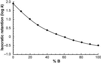
Unfortunately, it's not that simple. In the figure on the right, isocratic retention vs. eluent composition relationships are plotted for three different compounds.
Retention indexing assumes that a compound will always elute at the same position between two bracketing standards, but if you use the retention of amitriptyline and indole as bracketing compounds to predict the retention of acetophenone, it depends heavily on solvent composition; acetophenone doesn't even elute between amitriptyline and indole at some eluent compositions!
Since retention indexing can't account for variability in the retention vs. solvent composition relationships of different compounds, it can't account for any differences in the experimental conditions used in the experiment (e.g. the gradient program, the column dimensions, the flow rate, etc.). In fact, even relatively small, unintentional differences between HPLC systems (e.g. gradient delay, gradient dispersion, solvent misproportioning) can cause considerable error.
Retention "Projection"
Still, the isocratic retention information shown in the previous figure can be easily measured, so another approach to predicting gradient retention is to calculate it (or "project" it) from the isocratic retention data.
To explain how gradient retention times are projected from isocratic data, suppose for a moment that you measured the isocratic retention of a compound over a range of mobile phase compositions...
...and you want to calculate its retention time in the following gradient.
The easiest way to do it is to think of the gradient as a series of very short isocratic steps, each with a certain mobile phase composition.
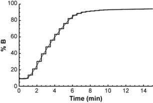
For each isocratic step, you could determine the compound's retention factor (from the isocratic retention vs. % B relationship above) and from that, calculate how far it will travel through the column during the step. After a number of isocratic steps, the compound will eventually have traveled the entire length of the column.
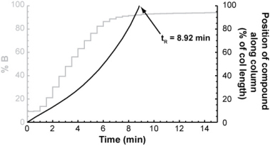
The number of isocratic steps it took to elute the compound multiplied by the length of each step gives its gradient retention time.
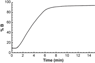
Unfortunately, this approach, by itself, isn't very accurate either (typically >10% error) because the actual gradient produced by an HPLC instrument isn't exactly what you program it to produce. Actual gradients usually differ considerably from the expected ones. On the right, you can see two gradient profiles measured from two different HPLC instruments, both programmed to produce the same 5 min gradient. Such gradient distortions must be taken into account to accurately project retention.
Back-Calculating the Gradient
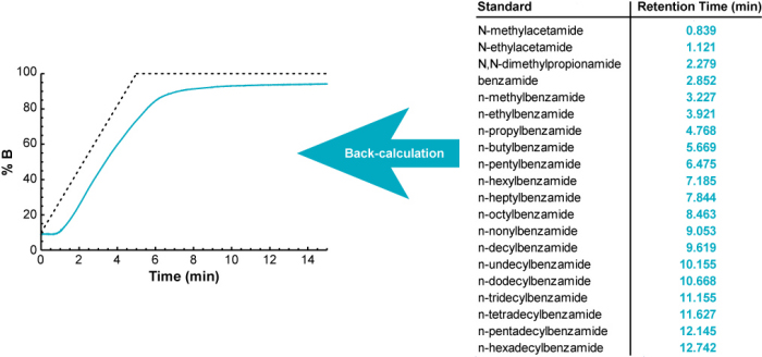
Rather than trying to directly measure the gradient, we discovered a much simpler, more accurate way to do it. We use the gradient retention times of a set of standards, spiked into the sample, to back-calculate what the gradient must have been to produce those retention times.
How does it do this? (click to expand)
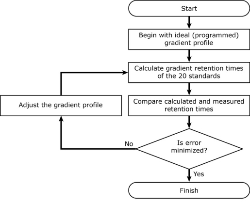
It uses an iterative process to back-calculate the gradient profile. It begins with the ideal (programmed) gradient profile, calculates retention times for each of 20 standards (using their known isocratic retention behavior; see below), and compares them with their measured retention times. Then it makes a small adjustment to the gradient profile, recalculates retention times for all 20 compounds, and checks to see if the accuracy of the calculated retention times improved. If so, it keeps the change, otherwise it discards it. It continues making small adjustments to the gradient profile until the difference between the measured and calculated retention times is minimized.
It turns out that this way of measuring the gradient is very accurate; when a back-calculated gradient is then used to project the retention of other compounds (for which their retention vs. solvent composition relationships are already known - see the retention database), the projected retention times are extremely accurate. The table below shows the measured and projected retention times of a set of chemically diverse compounds in a 20 min gradient at 400 uL/min. The root mean square error among all compounds was only ±1.0 s.
Chemical |
Measured Retention Time (min) |
Projected Retention Time (min) |
Difference (min) |
N,N-diethylacetamide |
3.817 |
3.817 |
0.000 |
N-allyl aniline |
4.394 |
4.409 |
-0.015 |
1,3-naphthalenediol |
7.322 |
7.29 |
0.032 |
diphenylamine |
12.989 |
12.97 |
0.019 |
coumarin |
5.774 |
5.78 |
-0.006 |
naphthalene acetamide |
7.082 |
7.07 |
0.012 |
2-phenylindole |
13.447 |
13.426 |
0.021 |
acetaldehyde |
11.087 |
11.079 |
0.008 |
tetrabutylammonium chloride |
8.93 |
8.929 |
0.001 |
abscisic acid |
7.192 |
7.203 |
-0.011 |
tetrapentyl ammonium bromide |
12.12 |
12.129 |
-0.009 |
prednisone |
7.494 |
7.496 |
-0.002 |
cortisone |
7.662 |
7.669 |
-0.007 |
hydrocortisone |
7.56 |
7.564 |
-0.004 |
curcumin |
11.76 |
11.799 |
-0.039 |
Not only is this method of predicting retention extremely accurate, but its accuracy does not deteriorate when the gradient, the flow rate, or the HPLC instrument is changed because it properly measures and accounts for the differences.
This approach offers three advantages over conventional HPLC retention databases:
1) It is extremely accurate. The back-calculation methodology accounts for unintentional differences between HPLC systems that would otherwise cause considerable error.
2) It remains accurate under a range of experimental conditions. One can change the gradient program, the flow rate, the column inner diameter, or the column length without losing accuracy.
3) It is easy to use and fast. You simply run your sample, spiked with 20 standards, and report their retention times to the open-source HPLC Retention Predictor application. You can even use the software to automatically extract them from the LC-MS data file.
The limitations of the methodology are:
1) At this time, you must use an Eclipse Plus C18 (3.5 µm particle size) column, though any column length or inner diameter is okay.
2) The column oven must be set to 35 °C.
3) The mobile phases must be 0.1% formic acid in water (solvent A) and 0.1% formic acid in acetonitrile (solvent B), prepared according to the procedure described in the Step-by-Step Instructions.
 Except where otherwise noted, all content on this site is licensed under a